How to Read an OTDR Trace: Events, Ghosts, Dead Zones

An OTDR trace is evidence, and like any evidence it has to be examined before it is believed. The instrument never measures loss directly. It fires light into the fiber and listens to the small fraction of it that scatters back — the Rayleigh backscatter — then infers loss from how that returning signal falls away with distance. Every feature you see — the slope, the steps, the spikes, the sudden drops — is the result of that inference, and every one of them can be produced by the fiber, by the instrument, or by the way the instrument was set up.

Technicians who read traces quickly are not faster at spotting spikes. They carry a short list of the ways a trace lies to people, and they check it in order. How to read an OTDR trace, then, is less a vocabulary exercise than a sequence of checks that decide whether the evidence in front of you is worth acting on — and knowing how to interpret an OTDR trace means knowing which of its numbers carry which error. This page is that list, followed by the decision it exists to support: is this link acceptable, and what exactly are you signing?

If you have not yet taken the measurement and want the instrument procedure that produces the trace — cleaning, launch cable, index of refraction, wavelength, pulse width — that is a separate job and it lives in how to test fiber optic cable. Everything below assumes a trace already exists. It sits under the wider installation, splicing and testing handbook for this part of the network.

The Trace Has Two Axes, and One of Them Is Already Approximate

The horizontal axis is distance, but nothing in an OTDR measures distance. It measures the round-trip time of a pulse and converts that to length using the group index of refraction you typed in, or the instrument guessed. Get the index wrong by 1 % and every distance on the screen is wrong by 1 % — 100 m of error on a 10 km span, which is the difference between "fault at the joint" and "fault 100 m past the joint" when a crew is digging.

There is a second offset that surprises people: the fiber is longer than the cable. The Fiber Optic Association's OTDR training material puts the fiber at roughly 1 % more than the cable length — the slack is there so the cable can stretch during pulling without straining the glass. A trace that reads 12.4 km is describing a route of about 12.3 km. On a long span that is a 100 m walk.

The vertical axis is returned signal power on a logarithmic scale, and the numbers you read off it are differences between two estimates of that power. That is why a trace is precise near the instrument and progressively less precise far away: the backscatter signal weakens with distance, the noise floor gets closer, and the same dB difference becomes harder to resolve. An attenuation reading taken across 5 km of clean fiber is a solid number. The same reading taken across 40 m, between two events, is mostly uncertainty.

Two habits follow, and they cost nothing:

• Measure attenuation only between two clean, straight sections. Marker placement is the whole method; a marker sitting on the curved shoulder after a reflective event is reading the instrument's recovery, not the glass.
• Never read a loss across an event. The slope before and after an event is the fiber; the step between them is the event. Mixing them gives a number that is neither.

How to Read an OTDR Trace: Four Shapes, Four Meanings

Almost everything on a trace is one of four shapes, and the shape tells you what kind of thing is there before you look at any number.

That last row is an incident rather than a measurement. A spike followed by nothing is either the end of the fiber or a break, and the trace tells you which by distance: if it is at the length you expected, it is the end; if it is short, something happened to the span, and the response from there is a restoration job rather than a reading exercise — how to repair a cut fiber optic cable picks it up at that point.

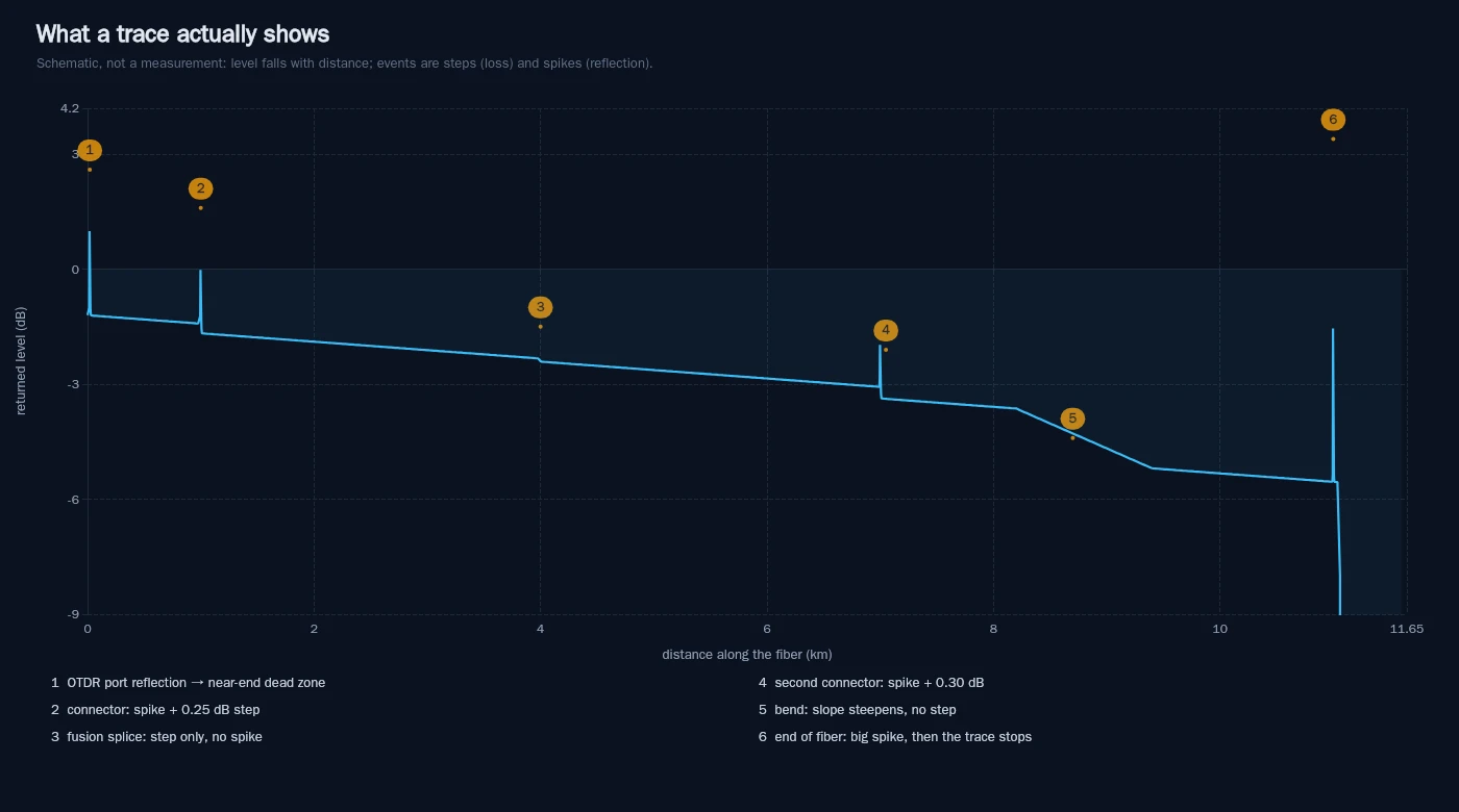
Schematic trace over an 11 km span. The slope is the fiber; the steps are events; the spikes are reflections. Not a measurement — the event losses shown are illustrative.

The discriminator between the first two rows is an air gap. A fusion splice fuses glass to glass, so almost no light reflects and you see only the loss. A mated connector almost always has a tiny gap or an index mismatch at the endface, which produces a Fresnel reflection — a spike — on top of the loss. That is why the same 0.3 dB can look completely different in two places on the same span, and why the choice between fusion splicing, mechanical splicing and connectorization shows up directly in the trace you are reading.

Angled physical contact changes the picture again. An APC endface is polished at an 8° angle, so the reflection leaves the core instead of traveling back to the detector. The connector is still there and still has loss, but it can look almost non-reflective — occasionally it disappears entirely at the resolution you are using. "I do not see a spike" is not the same claim as "there is no connector."

A bend is the quiet one. It removes light without reflecting any, so it reads as a stretch of fiber that attenuates faster than its datasheet says. Single-mode bends are wavelength-dependent: the same coil that looks acceptable at 1310 nm can be visibly lossy at 1550 nm. If a span passes at one wavelength and fails at the other, look at the routing before you look at the glass — the handling limits are set out in the bend radius rules.

Then there is the event table. Automatic event detection is a hypothesis, not a verdict. It merges events that are close together, it can miss a weak non-reflective step buried in noise, and it will happily label a ghost as a connector. Read the table as a list of candidates and confirm each one against the shape on the graph.

Why the Same Splice Reads Two Different Losses

Put two markers either side of a splice and let the instrument subtract the power levels: that is the two-point method, and on a short span it over-reads. The reason is simple — the distance between the markers contains fiber, and the fiber has loss. Move the markers closer and noise dominates; move them further apart and you are charging the splice for glass.

The fix is the least-squares approximation, usually shown as LSA. It fits a line to the backscatter on both sides of the event and extrapolates each line to the event's position, so the splice loss is the step between two fitted slopes rather than between two arbitrary points. Most modern instruments report LSA by default in the event table, and that is the number you should be certifying against. This is where most OTDR trace analysis goes wrong: the OTDR splice loss figure looks authoritative because it has two decimals, and its accuracy still depends entirely on which method produced it.

Two practical consequences:

1. A two-point reading and an LSA reading of the same splice are allowed to differ. On a short span the gap can be larger than the splice loss itself. If your number and the contractor's number disagree, check the method before you check the splice.
2. Two instruments will not agree to the third decimal. Different pulse widths, different fitting windows, different firmware. A 0.28 dB versus 0.31 dB argument across two OTDRs is measuring the instruments, not the joint. That is precisely why acceptance criteria carry a tolerance and why the acceptance test should name one instrument, one pulse width and one method.

A Negative Loss Is Not a Fault: Gainers and Backscatter Mismatch

Sooner or later a trace shows an event with a negative loss — the level after the event is higher than before it. New technicians read that as an OTDR gainer, a piece of hardware that somehow added light, and start looking for an amplifier. There is no amplifier. The backscatter coefficient of the two fibers is different.

Backscatter is not a constant. It depends on how much light the glass scatters per unit length, which varies with the fiber's core diameter, its doping and its attenuation. Splice a low-scatter fiber to a high-scatter one and more light comes back from the far side, so the OTDR, which is comparing returned power, sees the level rise. The splice can be perfect and still show a gainer; it can also hide real loss, because the arithmetic of the backscatter step cancels part of it.

There is exactly one honest fix, and it is not a setting: measure the link in both directions and average the two readings for each event. The backscatter error changes sign with direction, the splice loss does not, so the average removes most of it. Do not disconnect the launch and receive cables between the two passes — the point is to measure the same physical alignment twice, and re-mating the connectors creates a new event with a new reflectance.

An instrument that offers "bidirectional averaging" is doing that arithmetic for you from two saved traces. If yours does not, do it by hand: two files per fiber, averaged per event, both kept in the record.

Ghosts: How to Prove an Event Is Not There

A ghost is a reflection of a reflection — an OTDR ghost is light that bounced between two reflective ends more than once and came home late. When two reflective ends face each other — the launch-cable connector and the first connector of the link, for example — light bounces back and forth between them. Each bounce that escapes back toward the detector arrives later than the one before, so the trace grows events at regular intervals that correspond to no hardware at all.

The signature is arithmetic, and this is what makes ghosts provable rather than debatable:

• The distance is a multiple of the reflective span. A ghost sits at two, three or four times the length of the gap that created it — usually the launch cable or the first patchcord, and on a short span the cable under test is itself that gap. Divide the suspect event's distance by the distance to the strongest reflective event before it: a suspect event at 2.44 km with a launch-cable reflection at 1.22 km gives 2.0 exactly, and that is a ghost until proven otherwise.
• There is no loss step after it. A real event removes light permanently; the backscatter level after it is lower and stays lower. A ghost's returning pulse rides on the same backscatter level, so the trace returns to where it was.
• It disappears when you remove the reflection. Clean and re-mate the reflective connection, add index-matching gel at the far end, or swap in an angled endface — APC versus UPC matters here for exactly this reason. If the event vanishes and everything else stays put, it was never there.

The failure mode this prevents is expensive and well known. FOA's training material records a cable condemned as broken in the middle: the span was 40 m, a ghost appeared at 80 m and was read as the far end, so the real end at 40 m looked like a mid-span break — the tester never compared the distance scale against the cable's known length. A crew gets dispatched to a break that does not exist, and a cable that passes gets rejected. Ghosts cluster on short, highly reflective links: patchcord-heavy racks, short drop cables, anything where the reflection is strong enough to survive several bounces.

The settings matter too. A range set barely longer than the fiber, or a pulse so long that the events blur, makes ghosting worse; the Fiber Optic Association's guidance is to set the range to at least twice the fiber length, which is cheap insurance against both.

Dead Zones: What the Instrument Physically Cannot Show You

After a strong reflection the detector is temporarily blinded, the same way your eyes are after an oncoming headlight. Until it recovers, everything on the trace is unreliable — and "everything" means a specific, measurable stretch of fiber.

Two different limits get called an OTDR dead zone, and they answer two different questions. EXFO's application note on OTDR fundamentals defines them this way:

• Event dead zone — the minimum distance after a Fresnel reflection at which another event can be detected at all. Industry convention measures it at −1.5 dB either side of the reflective peak. Inside it, two events are merged into one entry with a combined loss.
• Attenuation dead zone — the minimum distance after a Fresnel reflection at which the loss of the next event can be measured accurately. It is measured until the trace returns to 0.5 dB above the fiber's backscatter level, and it is always longer than the event dead zone.

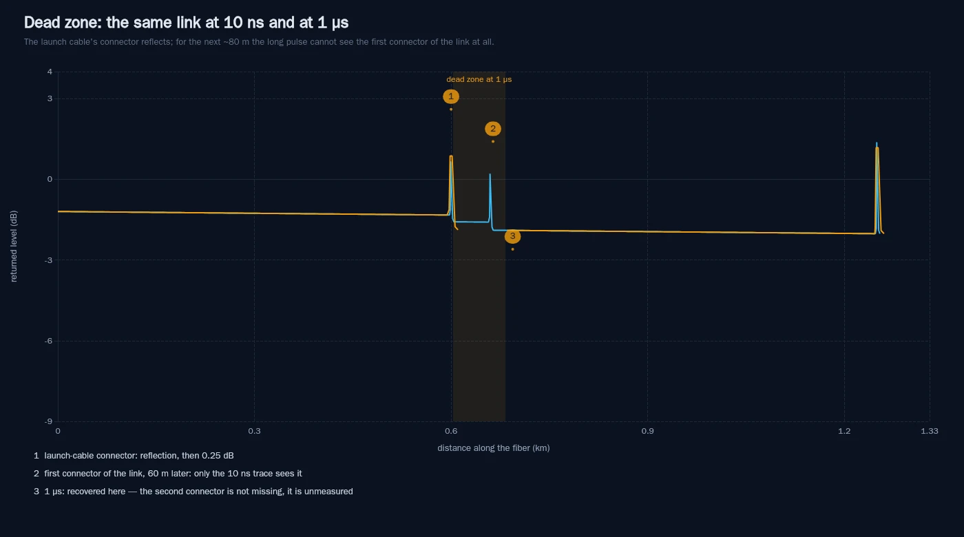
The same span at two pulse widths, with 600 m of launch cable in front of the link, which starts at the 0.60 km mark. At 1 µs the first connector of the link sits inside the dead zone: it is not "a clean connector", it is unmeasured.

That distinction explains a trace that confuses people: the second of two close connectors appears in the event table, so it was detected, but its loss is nonsense because it sits inside the attenuation dead zone. The pair in front of you is one measurement, not two.

Both dead zones stretch with pulse width. A short pulse resolves close events but carries little energy and dies early; a long pulse reaches the far end but swallows the first connectors. Reach itself is set by dynamic range — EXFO's rule of thumb is to pick a unit with 5 to 8 dB more dynamic range than the worst-case loss you expect, and it works an example: a 35 dB instrument has roughly 30 dB usable, which at 0.20 dB/km and a 0.1 dB splice every 2 km certifies about 120 km.

Read the footnotes before you compare two instruments. Dead zone specifications are quoted at the shortest available pulse and at a specified reflection — −45 dB for single mode, −35 dB for multimode is the common convention. A datasheet measured at −55 dB reflection will always look better, because a weaker reflection blinds the detector for less time. It is the same instrument physics measured under friendlier conditions.

The operational sentence to carry away is this: an event missing from the trace is a statement about the instrument, not about the fiber. A 30 cm patchcord between two connectors is invisible at most pulse widths. When you need to know what is inside the near field, use a visual fault locator, which finds the loss a tight bend or a bad connector leaks as visible red light, and which does not care about dead zones.

Judge the Trace Before You Judge the Fiber

Most wrong acceptance decisions are made before anyone looks at a loss number. The trace itself was not fit to judge, and nobody checked. Six things disqualify a trace:

1. A flat-topped spike anywhere near the events you care about. A saturated peak means the receiver was overloaded, and the loss readings immediately after it are recovery artifacts, not measurements.
2. No launch cable, or one too short. The first connector of the link sits inside the near-end dead zone and cannot be measured. The Fiber Optic Association recommends 500 m to 1 km, and any trace taken without a launch cable is missing its first event by construction.
3. Range shorter than twice the fiber. The trace distorts near the end and ghosts become likely, which is how a clean span gets rejected.
4. A noise floor reached before the end of the fiber. If the trace is still wandering when it stops, you have not seen the end — increase averaging or step up a pulse width and shoot again.
5. An index of refraction that does not match the fiber on the reel. Every distance is then wrong by the ratio of the two indices.
6. Multimode fiber shot with a laser-based OTDR treated as a loss certificate. More on that below.

Any one of these means: re-shoot, then judge. It is faster than defending a bad number to a client, and it is the cheapest way to avoid both wrong rejects and — much worse — wrong accepts.

The Pass/Fail Call: Three Checks, In This Order

Once the trace is trustworthy, the decision takes three checks. They answer three different questions, and a link only passes if all three do.

Check 1 — every event, individually. This is where per-event acceptance criteria apply, and they are tighter than most people assume:

That last row matters more than it did five years ago. Reflectance is the amount of light reflected at an event, expressed as a negative number, and the OTDR's reflectance reading is the same physical quantity as return loss expressed the other way round — closer to zero is worse. Where a link's insertion-loss budget used to be set by fiber type alone, short-reach single-mode applications now get different loss limits depending on the reflectance class of their connectors: Fluke Networks works the example straight out of the IEEE tables, where four connectors in the −45 to −55 dB class set a 3.0 dB insertion-loss limit and four in the −35 to −45 dB class set 2.7 dB. A link can pass its loss test and still fail on reflectance, and only the trace shows you where. The relationship between the two numbers is worth getting straight before the acceptance meeting; insertion loss versus return loss covers it in full.

Check 2 — end to end, against the budget that was written before the test. Add the fiber attenuation over the measured length, every splice, every connector pair and every splitter, and compare the total with the loss budget for the application, with the design margin still intact. A trace that passes every event and still exceeds the budget is telling you something useful: the budget assumed fewer connectors, a shorter route or a different fiber than the one that got installed. Re-shooting will not change it. The budget is a document you can rebuild and re-run — the fiber loss budget calculator does the arithmetic with splices and connectors as separate lines, which is the only way to see which line is eating the margin.

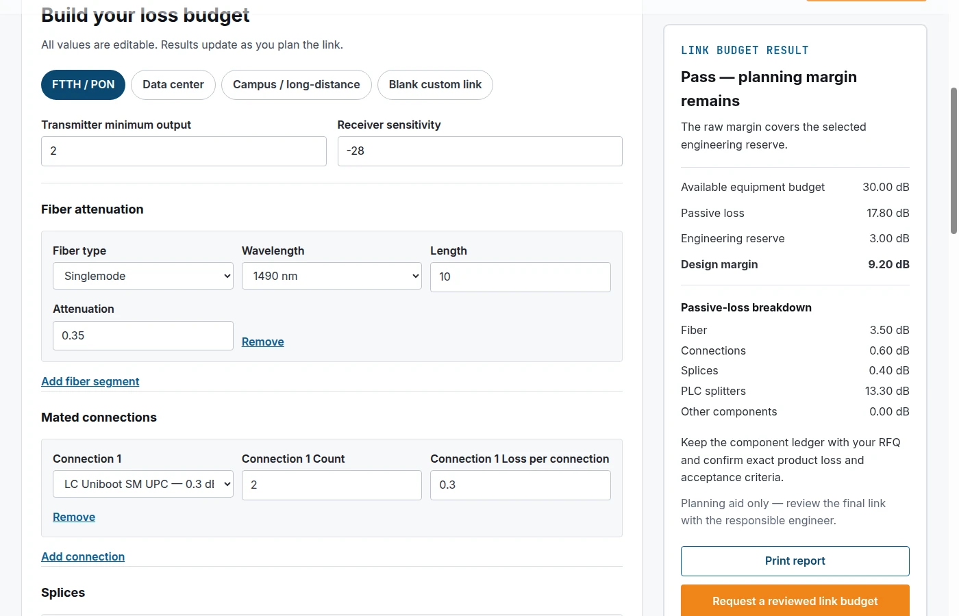
The budget the trace is judged against should be a written ledger with its own line for splices and connectors — otherwise "it passes overall" hides which line consumed the margin.

Check 3 — does the OTDR agree with the power meter? These are different measurements, and acceptance frameworks split the work the same way: Fluke Networks' OLTS and OTDR testing guide describes the power-meter pass as Tier 1 under TIA, with the combined OLTS + OTDR pass called Tier 2 (ISO/IEC calls it extended testing). Neither substitutes for the other — that is the point of making it a tier of its own. The OTDR infers loss from backscatter and reports each event; a light source and power meter measures what actually arrives. On a single-mode link the two end-to-end numbers should agree to within a few tenths of a dB as a matter of field convention; a larger gap is a setup problem — wrong launch, dirty reference, wrong wavelength, an uncorrected gainer — long before it is a cable problem.

When the three checks disagree, resolve them in this order: a failed event is a defect no matter what the total says; a failed total with clean events is a budget or design question; a disagreement with the power meter means the trace gets re-shot before anyone argues about the fiber. And whatever the outcome, write down the criteria you judged against. "PASS" without the criteria, the wavelength and the pulse width is not a result — it is an opinion with a number attached.

Two Traces That Break the Rules: Splitters and Multimode

Two plant types make the standard reading procedure produce nonsense, and both are common.

Through a PON splitter. A 1:8 PLC splitter removes about 9 dB before any excess loss — 3 dB per doubling, three doublings — so the trace shows a large downward step that is not a fault, and beyond it the backscatter from the drop side is often at or below the noise floor at the pulse width that resolved everything before the splitter. What you see after the splitter is frequently the splitter's own reflection and noise, not the drop fibers. Test from the splitter outwards, or use the splitter's own test port if it has one; the split ratio and the port losses are properties of the PLC splitter, not of the span. Reading a drop-side trace as if it were a point-to-point span produces the classic error of "the last 400 m are broken" when the truth is "the last 400 m are unmeasurable at this setting".

On multimode. An OTDR launches a narrow cone of light into the center of a multimode core; the LED sources these links were designed around fill the core. The center of the core has lower loss than the edges, so the OTDR under-reads. The Fiber Optic Association reports its own experience plainly: a multimode plant that measures 10 dB on a source and power meter can read 6–7 dB on an OTDR. An OTDR is still the right tool for multimode length, event location and reflectance, and the wrong tool for a multimode loss certificate. Certify multimode with the power meter and use the trace for geography.

What Has to Be in the Trace File

A trace that exists only on the instrument's screen has no value after the technician leaves. The file is what makes the next fault fast to find, and it is also what makes this acceptance defensible a year later. At minimum, each fiber's record should carry:

• wavelength, pulse width, range, averaging time and index of refraction used;
• launch and receive cable identifiers and lengths;
• both directions, saved separately, and the bidirectional average if your instrument can produce one;
• the event table with distance, individual loss, reflectance and cumulative loss;
• the measured attenuation in dB/km and the optical return loss for the link;
• the acceptance criteria document that was applied — including per-event limits;
• instrument model, serial number and last calibration date.

The most useful line in that list is the one nobody bothers with: the as-built baseline. Absolute numbers drift with instruments, pulse widths and firmware; a comparison to the trace taken the day the link was accepted does not. When a link starts failing two years later, the question is never "is 0.4 dB bad", it is "was this 0.4 dB there on day one".

There is a hardware half to this too. A trace can only be checked against numbers that exist, and passive assemblies are increasingly bought with insertion-loss and return-loss data reported per assembly. Assemblies specified that way give the acceptance call something to test against, and they are also what makes a per-event limit enforceable instead of aspirational. Our FTTH cabling range ships 100 % pre-shipment tested, with insertion and return loss verified on every assembly — which is the part of this page a manufacturer can honestly contribute: no instrument will fix a link that was never specified.

Quick Answers for the Field

Why does my trace show a negative loss?

Almost always a backscatter mismatch between two different fibers, not a gain. Confirm by measuring the same event from the other end; if the gainer flips to a positive loss, it is a gainer, and the bidirectional average is the number you keep.

Why can't I measure the first connector?

It sits inside the near-end dead zone created by the reflection at the OTDR port. A launch cable moves that reflection away from the connector you care about — which is its real job, not "pulse suppression".

Is this spike a real event or a ghost?

Check three things: is the distance a multiple of the nearest strong reflective span, is there a loss step after it, and does it disappear when the reflection is reduced with index-matching gel or an APC patchcord. Multiple, no step, disappears: ghost.

Does a passing OTDR replace the power meter?

No. They answer different questions, and mature acceptance testing runs both — a light source and power meter for the end-to-end number, an OTDR for where the loss is and what the reflectance is. On multimode, the power meter is the only one of the two that certifies loss.