FTTH ODN Design: Centralized vs Cascaded Splitting, and How to Choose

FTTH ODN design is the work of deciding where the optical split happens, how much fiber runs to each of those points, and what sits in the enclosure at each boundary. It is the part of optical distribution network design that cannot be fixed later with a firmware update: the splitters, cables and closures you choose are in the ground for fifteen years. Everything else in the passive network — cable counts, cabinet sizes, splice closures, test procedure, the cost per home passed — follows from that one placement decision.

Two patterns cover almost every residential build. In centralized splitting, one splitter serves a group of subscribers from a single location, and a dedicated fiber runs from that splitter to each home. In cascaded splitting (also called distributed or two-stage splitting), the split is divided between two points: a coarse split in the cabinet, a finer split closer to the homes. They are not better and worse versions of each other. They spend different things — fiber and duct on one side, loss points and fault surface on the other — and the right answer is set by density, route type, take-up profile and how much optical margin you are willing to leave unspent.

What an FTTH ODN Design Actually Fixes

The optical distribution network is the passive path between the OLT's PON port in the central office and the ONT at the subscriber. In FTTH network architecture terms it is the whole middle: everything between the two powered ends, carrying light nobody regenerates. No powered device sits in it: splitters, closures, cabinets, terminals and cable, nothing else. That passivity is the point of a PON, and it is also why ODN mistakes are permanent in a way that electronics mistakes are not — you can swap a line card in an afternoon, but re-splitting a neighborhood means new cable, new enclosures and new splicing.

Four decisions do most of the damage if they are wrong, and all four are cheap to change on paper in week one:

The rest of this guide works through those four in the order a design actually meets them. If you need the layer beneath — what a PON is and why one laser serves many homes — the FTTH deployment guide covers the architecture, and what a PON is covers the shared-medium mechanics.

The Three Segments, and Why the Acronyms Matter

Every ODN, however it is split, breaks into the same three cable segments. The boundaries between them are where hardware lives, and the acronym soup that surrounds FTTH is mostly a naming problem at those boundaries.

• Feeder — from the OLT, through the optical distribution frame (ODF) in the central office, to the first splitter location. One feeder fiber per PON port, or a small bundle reserved for growth.
• Distribution — from the splitter location to the access points near the subscribers. This is the segment whose fiber count the splitting decision controls.
• Drop — from the access terminal to the ONT at the premises. One drop per connected home, and the segment where installation labor concentrates.

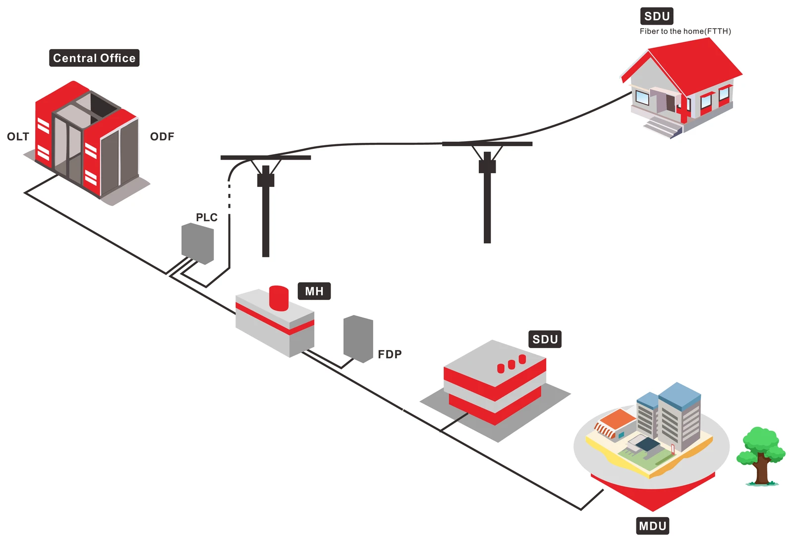
DYS reference architecture: OLT and ODF in the central office, a PLC splitter in the outside plant, then FDP and terminal points feeding single-dwelling and multi-dwelling premises.

The same physical box carries different names depending on which side of the industry you sit on, and half the confusion in a design review comes from two people meaning the same enclosure. A working map:

The component roles behind those names are worth ten minutes if the acronyms are still slippery: OLT vs ONU vs ONT vs ODN sets out which part is active, which is passive, and where responsibility changes hands.

Why insist on the naming? Because the splitting decision is a decision about which boundary holds the splitter, and that determines everything the enclosure at that boundary must contain: splitter ports, splice trays, adapter panels, slack storage, and the reserve fiber you promised the planning team.

Centralized Splitting: One Split Point, One Place to Test

Centralized splitting places the whole ratio in one location — the central office, or an ODC serving a few hundred homes. A 1:32 splitter takes one feeder fiber in and presents 32 ports out, each with its own distribution fiber running to a terminal near a home.

What it buys:

• One place to test and re-patch. Every splitter port is accessible at the same panel. A fault on one subscriber's distribution fiber can be isolated and re-patched without entering a single handhole, and an OTDR can be shot down any one branch from the cabinet because the branches are physically separate — the trace-reading method is the one in how to read an OTDR trace.
• Uniform optical loss. Every subscriber sees the same splitter loss and roughly the same fiber length, so one budget calculation covers the whole footprint and the weakest subscriber is predictable rather than discovered.
• Simple capacity accounting. Ports equal subscribers, one to one. Take-up forecasting becomes arithmetic instead of a puzzle.
• A clean upgrade path. If the PON moves from GPON to XGS-PON, the passive plant does not move — the splitters and distribution fibers stay where they are. The OLT optics and every ONT change, and a coexistence combiner installed alongside the GPON port adds its own loss.

What it costs:

• Fiber. 32 subscribers need 32 distribution fibers. A 1:32 centralized design with 1,000 homes passed behind it is 1,000 fibers of distribution cable to build, whether or not those homes ever connect.
• Duct and cable diameter. Those fibers occupy duct, weigh on aerial strand, and need splice closures sized for them.
• Longer average runs. The split point is far from the subscriber by construction, so the average drop-plus-distribution length is longer than in a cascaded design.

Centralized is the natural pattern for dense urban blocks and MDUs with a serviceable riser, where duct is available and take-up is expected to be high. When the fiber per subscriber is affordable, the operational simplicity is worth paying for.

Cascaded Splitting: Moving the Split Toward the Subscriber

Cascaded splitting divides the ratio between two points: a coarse split in the cabinet, a fine split at or near the access terminal. A 1:4 at the ODC followed by a 1:8 at the FAT is a 1:32 network — the ratios multiply, as the Fiber Optic Association's FTTx architecture reference puts it: a 4-way splitter followed by an 8-way splitter is a 32-way split.

What it buys:

• Fiber where it is expensive. The distribution cable now carries four fibers instead of 32 to reach the same 32 subscribers. Twenty-eight fewer fibers per group, multiplied across a suburb, is a different cable, a different duct fill, and a different splice closure.
• Staged investment. The first-stage splitter is sized for the area; the second-stage splitters are installed as homes connect. Capital follows take-up instead of anticipating it.
• A fit for scattered clusters. Where homes are grouped in small pockets along a rural route, a splitter at each pocket costs less than hauling dedicated fibers to all of them.

What it costs:

• More loss points, not more split loss. This is the part that surprises people. A 1:4 plus a 1:8 consumes 7 + 11 = 18 dB, exactly what a single 1:32 consumes. What the cascade adds is the second enclosure: another splitter, and another connection on every path — one mated pair if the second-stage splitter is spliced into the distribution fiber, two if it is connectorized at both ends (about 0.5 dB versus 1 dB). Each of those is also a place to fail.
• Unequal subscriber paths. A subscriber served by the first FAT on the route and one served by the last do not see the same loss. The design must be checked against the worst case, not the average.
• Fault domain. A splitter or a cut in the cabinet now affects everyone downstream of that branch rather than one subscriber.
• Testing discipline. An OTDR trace from the OLT through two splitters returns a composite of many branches; branch-level fault location needs testing from the FAT outward, or a tester that can see through splitters.

The pattern fits suburban and rural builds, aerial plant where cable weight matters, and any rollout where take-up is uncertain enough that pre-provisioning 32 fibers per group would be capital spent years early.

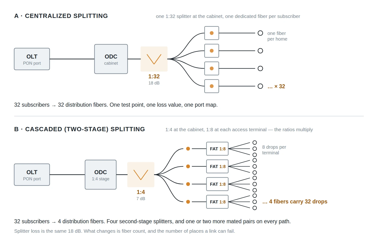
The same 32 subscribers, twice. Centralized: 32 dedicated distribution fibers from one splitter. Cascaded: 4 distribution fibers, each split again at the access terminal — a second layer of enclosures, and one or two more mated pairs on every path.

The Loss Budget That Decides Which Design Survives

Splitting arguments are settled by arithmetic, and the arithmetic starts with the splitter. Each stage of splitting costs optical power, and the numbers are not subtle:

Values from the FOA FTTx architecture reference; they include excess loss and are the numbers to design against, not the theoretical 3.01 dB-per-doubling figure.

Now put a splitter inside a real subscriber path. GPON optics are specified in budget classes — class B+ allows 28 dB and class C+ allows 32 dB, per ITU-T G.984.2, the physical media dependent layer of the GPON family defined in G.984.1. A class B+ design with a 1:32 splitter looks like this:

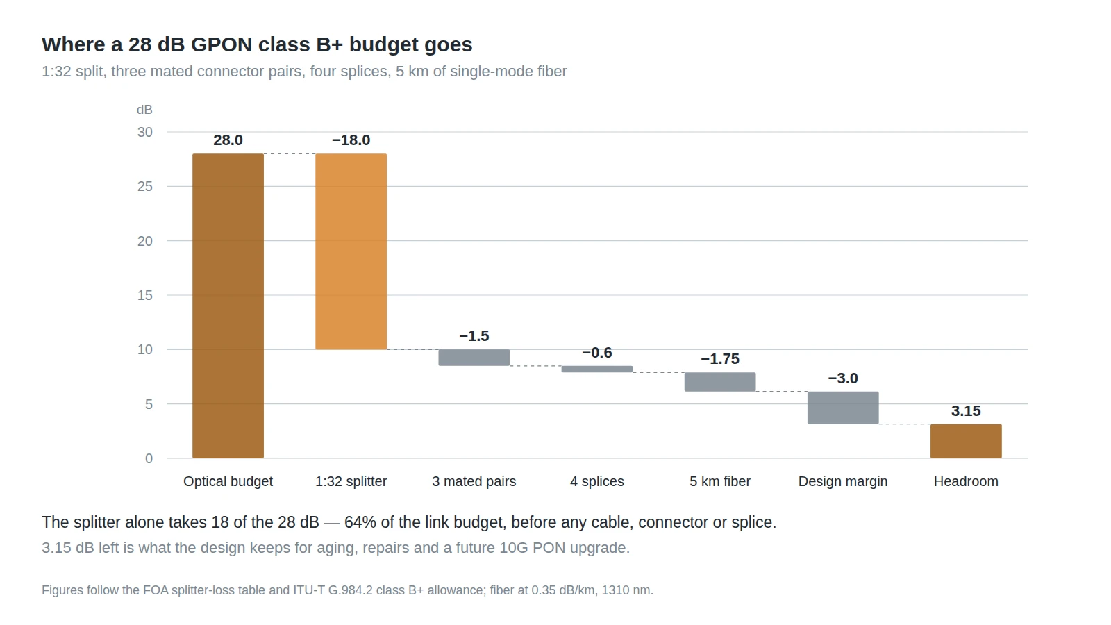
The same arithmetic as the table: a 28 dB class B+ budget with a 1:32 split, three mated pairs, four splices and five kilometers of fiber leaves a little over 3 dB of headroom.

Three things follow, and they decide the architecture more often than any preference does.

The split ratio is the largest single line. At 18 dB it consumes 64% of a class B+ budget before a single connector is counted. Moving from 1:32 to 1:64 costs another 3 dB, which is roughly the margin of a well-built short-reach design — so a 1:64 design has to buy that 3 dB somewhere: shorter reach, fewer splices, class C+ optics, or a pre-connectorized route that eliminates field splices.

The cascade does not cost split loss, it costs terminations. Because 1:4 + 1:8 equals 1:32 in dB, the difference between the two architectures in the budget is the second enclosure's connections — about 0.5 dB with a spliced splitter input, up to 1 dB if both the input and the output are connectorized. That is the honest way to compare them: cascaded splitting is not an optical penalty, it is an operational one.

Budget the worst subscriber, not the average. In a centralized design that distinction is small. In a cascade, the subscriber at the end of the longest distribution run behind the deepest second-stage splitter defines whether the design passes. If the average path has 7 dB of headroom and the worst has 1 dB, the design has 1 dB.

That margin also has a second job. XGS-PON budgets run from 29 dB (class N1) through 31 dB (N2) and 33 dB (E1) to 35 dB (E2) under ITU-T G.9807.1, and the optics that deliver 10 Gbit/s symmetric are less forgiving of a marginal path than GPON optics. A design that spends every spare decibel on a longer reach or a deeper cascade is a design that cannot take the upgrade without re-splitting. Keeping 3 dB in hand is how an ODN survives its second life.

Split Ratio: What the Ratio Buys and What It Costs You

The ratio is a commercial decision disguised as an optical one. It sets how much of the PON's capacity each subscriber can be sold.

A GPON port carries 2.488 Gbit/s downstream and 1.244 Gbit/s upstream. Split 32 ways, the downstream average is about 78 Mbit/s per subscriber if everyone is active at once; split 64 ways, it is about 39 Mbit/s. XGS-PON at 9.95 Gbit/s symmetric turns those into roughly 311 and 156 Mbit/s. Nobody is active all the time, and PON statistics are kinder than the average suggests — but the average is the number to quote when a wholesale customer asks what the split guarantees.

The design consequence is a rule of thumb that holds across vendors: choose the deepest ratio the loss budget can carry, then check that the resulting share still sells. In practice that means 1:32 for GPON in most residential builds, 1:64 where reach is short and take-up is expected to stay low, and 1:64 as the common starting point for XGS-PON where the 10 Gbit/s port makes the deeper split affordable. The generation-by-generation differences are set out in GPON vs XG-PON vs XGS-PON.

One warning on ratio arithmetic: it is tempting to plan a 1:64 split and then discover the second-stage splitter cannot be installed inside the FAT you specified. Splitting ratios constrain hardware, not the other way around — the enclosure's port count and splitter format must be chosen with the ratio already fixed.

Choosing Between Them: A Decision Sequence

Five questions, asked in this order, resolve most designs. The order matters because the first two are physical and cannot be argued with, while the last three are commercial and can.

1. How many homes sit within a sensible drop length of one access point? PON splitter placement follows density before anything else: if the answer is "thirty or more in one block", centralized is available. If it is "six here, eight there", a second-stage split is the only way to avoid hauling fiber to each pocket.
2. What is the route? Aerial plant rewards cascaded designs because cable weight and strand loading are real constraints. Duct-rich urban plant removes that pressure and makes centralized fiber affordable.
3. What take-up do you actually expect in years one to three? Centralized pre-provisions every subscriber; cascaded installs the second stage as homes connect. If take-up is uncertain, cascaded moves capital later.
4. Can you test and operate what you build? Every extra splitter stage and enclosure is a truck roll and a test procedure. An operator with a strong field-test culture and good records can run a cascade; one without will find centralized designs cheaper to keep alive.
5. What is the upgrade plan? If XGS-PON is on the roadmap within the asset life, check the cascade's worst-case path against the 29 dB class N1 budget before committing.

Hardware That Has to Match the Splitting Plan

The splitting plan only becomes real in hardware, and three items carry most of the risk.

Splitter packaging. The same 1:32 planar lightwave circuit sits in very different packages: an LGX cassette for a rack in the ODC, an ABS box for a FAT or pedestal, a steel-tube module for splicing directly into a closure, and hardened outdoor housings for direct burial. Choosing the ratio before choosing the package is the usual order; choosing the package before checking the enclosure's internal depth is the usual mistake.

Enclosures sized on working plus reserve. A FAT specified for eight working drops and no reserve is full on the day the ninth neighbor asks for service. Size on working ports plus the reserve policy — typically 20–30% — and count adapter ports, splice trays and cable entries separately rather than applying one maximum number to every product.

Connectors and fiber type at the drop. PON links carry a splitter, so reflectance matters and angle-polished (APC) interfaces are the norm in the ODN. The drop itself should be bend-insensitive single-mode — ITU-T G.657 fiber, specified at 10 mm bend radius for the A1 sub-class, 7.5 mm for A2 and B2, and 5 mm for B3 — because the last thirty meters of any residential build go around corners nobody drew. The practical limits are in fiber optic bend radius rules.

The hardware layer is where a design either scales or accumulates exceptions. DYS manufactures the ODN components this decision lands on — PLC splitters in cassette and ABS-box formats, terminal and HUB boxes for the access and distribution points, and flat or self-supporting drop cable — so a split plan can be quoted as one bill of materials rather than assembled from four suppliers. If you are specifying a build, send us the split plan and route and we will quote against it.

Mistakes That Surface Three Years After Handover

These are the ones that look harmless in a design review and expensive in year three.

• Sizing enclosures on working fibers only. Reserve is not a luxury; it is what makes the ninth connection a patch rather than a rebuild.
• One split ratio across a whole footprint. Dense blocks and scattered rural pockets have different economics. A single ratio serves neither well.
• Designing to the average path. In a cascade, the worst subscriber is the design.
• Counting the splitter and forgetting the terminations. Two extra mated pairs per subscriber is about 1 dB — a third of the three-decibel margin a class B+ design holds.
• Spending the margin on reach. Every decibel used to stretch a link is a decibel unavailable for the 10G upgrade.
• Splitters documented by ratio, not by port map. "1:32 at cabinet 14" is not a record. Which port serves which address is.
• Mixing polish types. APC in the ODN and UPC at the ONT is a 0.3 dB surprise and a reflectance problem, not a rounding error.

ODN Design Questions Planners Ask

What is the difference between centralized and cascaded splitting? Centralized puts the whole ratio in one place — a 1:32 splitter in the cabinet, one dedicated fiber per subscriber from there. Cascaded divides the ratio between two places — a 1:4 in the cabinet and a 1:8 at the access terminal, which multiplies to the same 1:32. The optical budget is nearly identical; the fiber count and the number of field enclosures are not.

Does cascaded splitting cost more loss? Barely. A 1:4 plus a 1:8 is 18 dB, the same as a single 1:32. The extra cost is the second enclosure's connections — about 0.5 dB with a spliced splitter input, up to 1 dB if it is connectorized at both ends — plus an unequal loss spread between the nearest and farthest subscriber.

What split ratio should an FTTH ODN design use? The deepest ratio the budget can carry that still sells the service you promise. For GPON residential builds that is usually 1:32; 1:64 appears where reach is short and take-up is low, or where the PON is XGS-PON and the 10 Gbit/s port absorbs the deeper split.

What is an ODN loss budget? The sum of every loss a signal meets between the OLT and the ONT — splitters, connectors, splices, fiber attenuation — compared against the optical budget of the PON class in use. Class B+ allows 28 dB, class C+ 32 dB, XGS-PON class N1 29 dB.

What is the difference between an ODC and a FAT? The ODC (or FDH) is the cabinet where feeder fibers terminate and the first split usually happens. The FAT (or FDP, or MST) is the smaller terminal near the homes where distribution fibers end and drop cables begin. A centralized design has splitters in the ODC; a cascaded design has them in both.

Can I run 1:64 on GPON? Yes, if the loss budget allows it and the per-subscriber share still sells — but 1:64 spends 21 dB of a 28 dB class B+ budget before terminations, which leaves very little for reach, splices and margin. Most 1:64 GPON designs are short-reach and pre-connectorized for that reason.